Odds Generation — point · quarter

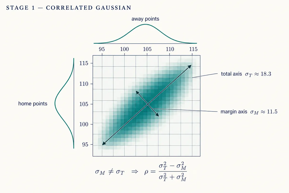
Enter the full match's Handicap and Total quotes in Malay and its Moneyline in decimal — margins still embedded in all three. Basketball is not Poisson: shared pace correlates the two teams' scores, so the margin and the total carry different dispersions (σ_M ≈ 11.5 vs σ_T ≈ 18.3 in the NBA) where one Poisson rate would force them equal. The engine (ADR-029):

1. strips each bookmaker margin (Power method — all three books are two-way) to fair probabilities;
2. back-solves a correlated-Gaussian score grid — the Total fixes μ_T, the Handicap fixes μ_M, and the Moneyline fixes the margin dispersion σ_M (a fixed spread's ML price is pure dispersion information); σ_T stays a league prior and the team correlation ρ falls out derived;
3. refines the grid in fixed stages — the plain Gaussian baseline, then the regulation-tie inflation ι (trailing teams play for the tie — the Dixon-Coles analog), then the ML σ fit (toggle in the Moneyline box); full-match markets settle including overtime, so tie cells fold through an OT mini-grid and the settlement margin is never 0;
4. derives quarters and halves from the solved match by Brownian √t scaling — variance takes the time share, drift takes calibrated shares (the home edge front-loads into Q1, Q4 scores least) — and prices every market below off the pipeline's last stage.

Stage 1 — shared pace tilts the score cloud: the total axis carries σ_T ≈ 18.3, the margin axis σ_M ≈ 11.5, and ρ = (σ_T² − σ_M²)/(σ_T² + σ_M²) falls out derived

Each stage re-solves the same fair targets, so the score grid's stage switcher is a true before/after — flip Gaussian / Tie ι / ML σ to see exactly what ι and the Moneyline move.

Unlike goal · regular, the sub-periods here are derived, not separately quoted — that is the point: three full-match quotes generate the whole quarter/half sheet (a period with its own quotes would simply be its own inversion). Markets needing basket order or timing (First/Last Basket) are out of scope for a score grid; see the Markets reference.

Handicap quote (Malay) — full match

LineHomeAway

Total quote (Malay) — full match

LineOverUnder

Moneyline (Decimal) · σ from ML

Homeincl. OTAwayincl. OT

Shape priors · margins

σ_Tleagueσ_Mpre-MLι (tie)diag ×ιMulti-wayShinTwo-wayladder

Quarter shares % (μ drift · total)

w_M Q1Q2Q3Q4w_T Q1Q2Q3Q4

↑/↓ steps a field, Shift steps bigger; on a Malay pair the partner moves the opposite way. Quotes are the full match (incl. OT); quarters and halves derive by √t scaling with the share knobs — normalized to 100% on use.

Valid inputs: Malay in [−1, +1] and never 0, decimals above 1, each book carrying margin, σ_T > σ_M (shared pace ⇒ ρ ≥ 0), ι in (0.5, 3.5).

μ_M 6.6663μ_T 224.6662σ_M 11.4092ρ 0.4489OT 4.6%round-trip Δp 1.8e-8 / 2.2e-8 / 1.6e-7grid N=229 · Gaussian → Tie ι → ML σ

Score grid — P(home ∈ bin, away ∈ bin) ×100 · bins of 5

μ_M 6.67μ_T 224.67σ_M 11.41σ_T 18.50OT 4.6%

	A=70	A=75	A=80	A=85	A=90	A=95	A=100	A=105	A=110	A=115	A=120	A=125	A=130	A=135	A=140
H=75	0.0	0.0	0.0	0.0	0.0	0.0	0.0	0.0	0.0	0.0	0.0	0.0	0.0	0.0	0.0
H=80	0.0	0.0	0.0	0.0	0.0	0.0	0.0	0.0	0.0	0.0	0.0	0.0	0.0	0.0	0.0
H=85	0.0	0.0	0.0	0.1	0.1	0.1	0.1	0.1	0.0	0.0	0.0	0.0	0.0	0.0	0.0
H=90	0.0	0.0	0.1	0.2	0.2	0.4	0.3	0.2	0.1	0.1	0.0	0.0	0.0	0.0	0.0
H=95	0.0	0.0	0.1	0.3	0.6	0.6	0.9	0.7	0.4	0.2	0.1	0.0	0.0	0.0	0.0
H=100	0.0	0.1	0.2	0.4	0.9	1.4	1.4	1.6	1.1	0.6	0.3	0.1	0.0	0.0	0.0
H=105	0.0	0.0	0.2	0.5	1.1	1.9	2.6	2.2	2.2	1.3	0.6	0.2	0.1	0.0	0.0
H=110	0.0	0.0	0.1	0.4	1.0	2.0	3.0	3.5	2.6	2.3	1.2	0.5	0.1	0.0	0.0
H=115	0.0	0.0	0.1	0.3	0.7	1.6	2.7	3.5	3.7	2.5	1.8	0.8	0.3	0.1	0.0
H=120	0.0	0.0	0.0	0.1	0.4	1.0	1.9	2.7	3.1	2.9	1.8	1.1	0.4	0.1	0.0
H=125	0.0	0.0	0.0	0.0	0.2	0.5	1.0	1.6	2.1	2.1	1.8	1.1	0.6	0.2	0.0
H=130	0.0	0.0	0.0	0.0	0.1	0.2	0.4	0.8	1.1	1.2	1.0	0.9	0.5	0.2	0.0
H=135	0.0	0.0	0.0	0.0	0.0	0.1	0.1	0.3	0.4	0.5	0.5	0.4	0.4	0.2	0.1
H=140	0.0	0.0	0.0	0.0	0.0	0.0	0.0	0.1	0.1	0.2	0.2	0.2	0.1	0.1	0.1
H=145	0.0	0.0	0.0	0.0	0.0	0.0	0.0	0.0	0.0	0.1	0.1	0.1	0.0	0.0	0.0

home lead near tie away leadsettlement grid — regulation ties already folded through OT

MarketHandicapOver/UnderHome Team Over/UnderAway Team Over/UnderMoneylineOdd/EvenWinning Margin (12 Way)Last Digit ScoreHome Team Last Digit ScoreAway Team Last Digit ScoreEnding Game11 in scope

settles including overtime — the OT fold leaves no tie mass

Outcome	Fair	Dec	Priced	Malay
Home	72.0%	1.388	1.358	+0.36
Away	28.0%	3.575	3.282	-0.44

How these numbers are computed

1 · Strip the bookmaker margins (Power method — all books are two-way)

A two-way Malay price converts to decimal ($d = 1 + m$ if $m > 0$, else $d = 1 - 1/m$), implying $q = 1/d$ with overround $Q > 1$; the Power method finds the exponent $x$ deflating the pair to fair $p_i = q_i^{1/x}$. The Moneyline is quoted in decimal, so it skips the Malay conversion but strips identically — basketball has no draw leg to Shin, the ML is a plain two-way book. These fair numbers are the three targets the solver must reproduce.

Handicap -6.50 → P(home covers -6.50)

	Home	Away
Malay quote	+0.96	+0.96
Decimal $d$	1.9600	1.9600
Implied $q = 1/d$	0.5102	0.5102
Fair $p = q^{1/x}$	0.5000	0.5000
Fair decimal $1/p$	2.0000	2.0000

overround Q = 1.0204 → solve $q_1^{1/x} + q_2^{1/x} = 1$ → x = 0.9709 → fair P(home covers) = 50.00%

Total 225.50 → P(over 225.50)

	Over	Under
Malay quote	+0.95	+0.95
Decimal $d$	1.9500	1.9500
Implied $q = 1/d$	0.5128	0.5128
Fair $p = q^{1/x}$	0.5000	0.5000
Fair decimal $1/p$	2.0000	2.0000

overround Q = 1.0256 → solve $q_1^{1/x} + q_2^{1/x} = 1$ → x = 0.9635 → fair P(over) = 50.00%

Moneyline (incl. OT) → P(home wins)

	Home	Away
Decimal quote	1.36	3.30
Decimal $d$	1.3600	3.3000
Implied $q = 1/d$	0.7353	0.3030
Fair $p = q^{1/x}$	0.7203	0.2797
Fair decimal $1/p$	1.3883	3.5751

overround Q = 1.0383 → solve $q_1^{1/x} + q_2^{1/x} = 1$ → x = 0.9372 → fair P(home ML) = 72.03%

Try the strips standalone — Margin — two-way (Power): the same math on any quotes, with the bisection narrated.

2 · Location — μ_T from the Total, μ_M from the Handicap

Model the two teams' points as a correlated bivariate normal, discretized to integer scores — each cell $(h, a)$ gets $P(H{=}h) \cdot P(A{=}a \mid H{=}h)$ with $P(k \in \text{cell}) = \Phi\!\big(\tfrac{k + 0.5 - \mu}{\sigma}\big) - \Phi\!\big(\tfrac{k - 0.5 - \mu}{\sigma}\big)$. Conditioning keeps parity exact ($T = M + 2A$ so total and margin are always odd or even together) — Odd/Even and Last Digit depend on it. Two location knobs match the first two targets:

$$P(\text{home covers } -6.50) = \Phi\!\Big(\tfrac{\mu_M - 6.50}{\sigma_M}\Big) \Rightarrow \mu_M \approx +6.50 + \sigma_M\,\Phi^{-1}(0.5000) = 6.5000$$$$P(\text{over } 225.50) = \Phi\!\Big(\tfrac{\mu_T - 225.50}{\sigma_T}\Big) \Rightarrow \mu_T \approx 225.50 + \sigma_T\,\Phi^{-1}(0.5000) = 225.5000$$

Those closed forms are only the seeds: full-match quotes settle including overtime, so the solver bisects each knob until the discretized, ι-tilted, OT-folded grid reproduces the fair targets exactly (final: $\mu_M = 6.6663$, $\mu_T = 224.6662$ — regulation-scoped, slightly off the seeds because OT adds points to tied games). Line rules are goal-regular's: a push refunds, fair = $W/(1-R)$; quarter lines split ½/½.

3 · Shape — σ_M from the Moneyline · ρ is derived

Poisson has one dial: it forces $\sigma_M = \sigma_T = \sqrt{\lambda_{\text{total}}} = \sqrt{224.67} = 14.99$. Basketball needs two — shared pace correlates the teams' scores, narrowing the margin and widening the total. The Total quote fixed μ_T but says nothing about σ_T (one line cannot identify a dispersion), so σ_T = 18.50 is a league prior knob. The Moneyline is the third anchor — at a fixed spread, the ML price is pure dispersion information (Polson & Stern's “implied volatility”):

$$P(\text{home ML}) = \Phi\!\Big(\tfrac{\mu_M}{\sigma_M}\Big) \Rightarrow \sigma_M \approx \tfrac{6.5000}{\Phi^{-1}(0.7203)} = \tfrac{6.5000}{0.5837} = 11.1360 \;\xrightarrow{\text{re-solve on the grid}}\; \sigma_M = 11.4092$$

The pair (σ_M, σ_T) is a complete reparameterization of the equal-variance bivariate normal — the team correlation and per-team dispersion fall out:

$$\rho = \frac{\sigma_T^2 - \sigma_M^2}{\sigma_T^2 + \sigma_M^2} = \frac{18.50^2 - 11.41^2}{18.50^2 + 11.41^2} = 0.4489 \qquad \sigma_{\text{team}} = \sqrt{\tfrac{\sigma_M^2 + \sigma_T^2}{4}} = 10.8676$$

ρ ≈ 0.3–0.5 is the empirical NBA pace band — the model recovers it from quotes alone. σ_T is the one number the three quotes cannot pin; alternate-total or team-total quotes would (ADR-029 O4 — the Methodology-B direction).

4 · Corrections — tie inflation ι, then the OT fold

A plain Gaussian underprices regulation ties: NBA games end regulation level ≈ 1.5–1.8× more often than the smooth curve predicts (trailing teams foul and shoot threes to force the tie; tied teams hold for the last shot). The fix is goal-regular's diagonal move — multiply every equal-score cell by ι and renormalize:

$$J[k][k] \mapsto \iota \cdot J[k][k] \quad (\iota = 1.60), \qquad \text{then } J \mapsto J / \textstyle\sum J$$

Full-match markets settle including OT, so the settlement grid folds each tie cell $(k, k)$ through an overtime mini-grid — the same bivariate machinery scaled to $f = 5/48$ of regulation ($\mu \cdot f$, $\sigma \cdot \sqrt{f}$) with the OT diagonal excluded and renormalized (a double OT — 10.6% of overtimes here — distributes like a single one). The settlement margin is never 0, which also skews totals slightly odd: P(odd) = 51.72% (parity ≡ margin parity). Every stage re-solves the same fair targets on its own grid:

Stage	μ_M	μ_T	σ_M	reg tie	Δ cover	Δ over	Δ ML
Gaussian	6.4445	224.9766	11.5000	3.0%	1.8e-8	1.8e-8	—
Tie ι	6.6646	224.6705	11.5000	4.6%	1.7e-8	1.6e-8	—
ML σ	6.6663	224.6662	11.4092	4.6%	1.8e-8	2.2e-8	1.6e-7

Flip the grid panel's stages to see what ι moves: the tie row is the OT rate, and markets near the spread feel the redistributed mass. ι is a calibrated league knob (like Dixon-Coles' ρ), spread- dependent in reality — the empirical NBA margin histogram (|margin| 1 depressed, 5–9 elevated) is the next correction of this kind, left as a data-calibrated reweight (ADR-029).

5 · Periods — Brownian √t slicing to quarters and halves

Scoring is empirically a random walk in time, so a period spanning share $v$ of the game takes $v$ of the variance — dispersion scales by $\sqrt{v}$ — while the drift takes calibrated shares: the home edge front-loads (≈ ⅔ of it lands in Q1) and Q4 scores least (garbage time beats the foul parade):

$$\mu_{M,q_i} = w^M_i\,\mu_M \qquad \mu_{T,q_i} = w^T_i\,\mu_T \qquad \sigma_{q_i} = \sigma \cdot \sqrt{\tfrac{1}{4}} = \tfrac{\sigma}{2} \qquad \text{halves: sum two quarters, } \sigma/\sqrt{2}$$

share	Q1	Q2	Q3	Q4
drift w_M	28.0%	24.0%	25.0%	23.0%
total w_T	25.4%	25.0%	25.5%	24.1%
margin drift μ_M·w	1.87	1.60	1.67	1.53
total mean μ_T·w	57.1	56.2	57.3	54.1

Period grids are regulation segments: no OT fold, and ties are real outcomes — a tied quarter pushes the 2-way moneyline, so its fair price renormalizes the tie away, $W/(1-R)$ (Q1 here: $R = 6.62\%$ tie mass → fair home = $63.68\%$). Pick a quarter or half above to see its grid and markets.

These weights are the calibration surface: fit w from your own results/odds history per league (ADR-029 O1). A period with its own quotes needs none of this — it is its own inversion, exactly like goal-regular's periods.

6 · Read “Moneyline” off the score grid

With the last stage fixed, the period grid $J[h][a]$ is fully determined and every market probability is a sum of its matching cells. Home sums every cell with home > away. A tied period pushes (stake refunded), so the fair two-way is W/(1−R); the full match settles through the OT fold, which leaves no tie mass.

Outcome	Fair	Priced dec
Home	72.0%	1.358
Away	28.0%	3.282

Fair probabilities are then priced with the Power ladder — $q_i = p_i^{\,x}$, bisecting $x$ until the pair's Malay-points gap hits 0.08 (this run: $x = 0.9330$). Same margin machinery as goal-regular — nothing basketball-specific here.

7 · Implementation notes — windows, bisection, normalization

targets   tC = powerStrip(HCP pair)       # fair P(home covers L)        — step 1
          tO = powerStrip(Total pair)     # fair P(over T)               — step 1
          tW = powerStrip(ML pair)        # fair P(home ML); ML stage    — step 3

stage ∈ {Gaussian (ι=1), Tie ι, ML σ}:    # each stage re-solves all targets
  sweep ×2 + polish:
    bisect μ_M   until P(cover L | grid) = tC     # grid = reg ± ι, OT-folded
    bisect μ_T   until P(over T | grid)  = tO
    bisect σ_M   until P(home ML | grid) = tW     # ML stage only
  grid: bivariate normal cells on a ±7σ window, diagonal ×ι, renormalize;
        tie cells fold through the OT mini-grid (f = 5/48, no OT diagonal)

periods: μ·w share, σ·√v (v = ¼ / quarter) → regulation grid, no ι, no fold

Every residual is monotone in its knob (cover ↑ μ_M, over ↑ μ_T, favourite ML ↓ σ_M), so plain bisection converges — the Δ's in step 4's table are this run's achieved errors. The window keeps each solver evaluation at ~20k cells (adjacent cells share a Φ boundary), and the renormalize absorbs both the window truncation and ι. Grids run 0..229 here; the pmf readers the solver uses are pinned to the grid readers the markets use by the test suite in docs/src/lib/odds/__tests__/basket.test.ts. Decision record: specs/adr/029-odds-generation-latent-parameter-reverse-engineering.md.