Odds Generation — goal · regular

Pick a period and enter that period's Handicap and Total quotes in Malay and its 1X2 in decimal — margins still embedded in all three. The engine:

1. strips each bookmaker margin (Power method for the two-way pairs, Shin for the three-way 1X2) to fair probabilities;
2. back-solves the period's goal rates (λₕ, λₐ) by nested bisection — the Total quote fixes how many goals, the Handicap quote fixes who scores them;
3. refines the score grid (the joint final-score distribution) in fixed stages — the independent-Poisson baseline, then Dixon-Coles' low-score correlation ρ (lifts draws and 0-0/1-1 at the expense of 1-0/0-1), then an optional diagonal lift φ that lands the draw mass on the 1X2 draw (toggle in the 1X2 box; off = the plain two-quote inversion);
4. prices every market below off the pipeline's last stage.

Stage 1 — the solved rates (λₕ, λₐ) outer-product into the joint score grid: P(h,a) = P(h;λₕ) · P(a;λₐ)

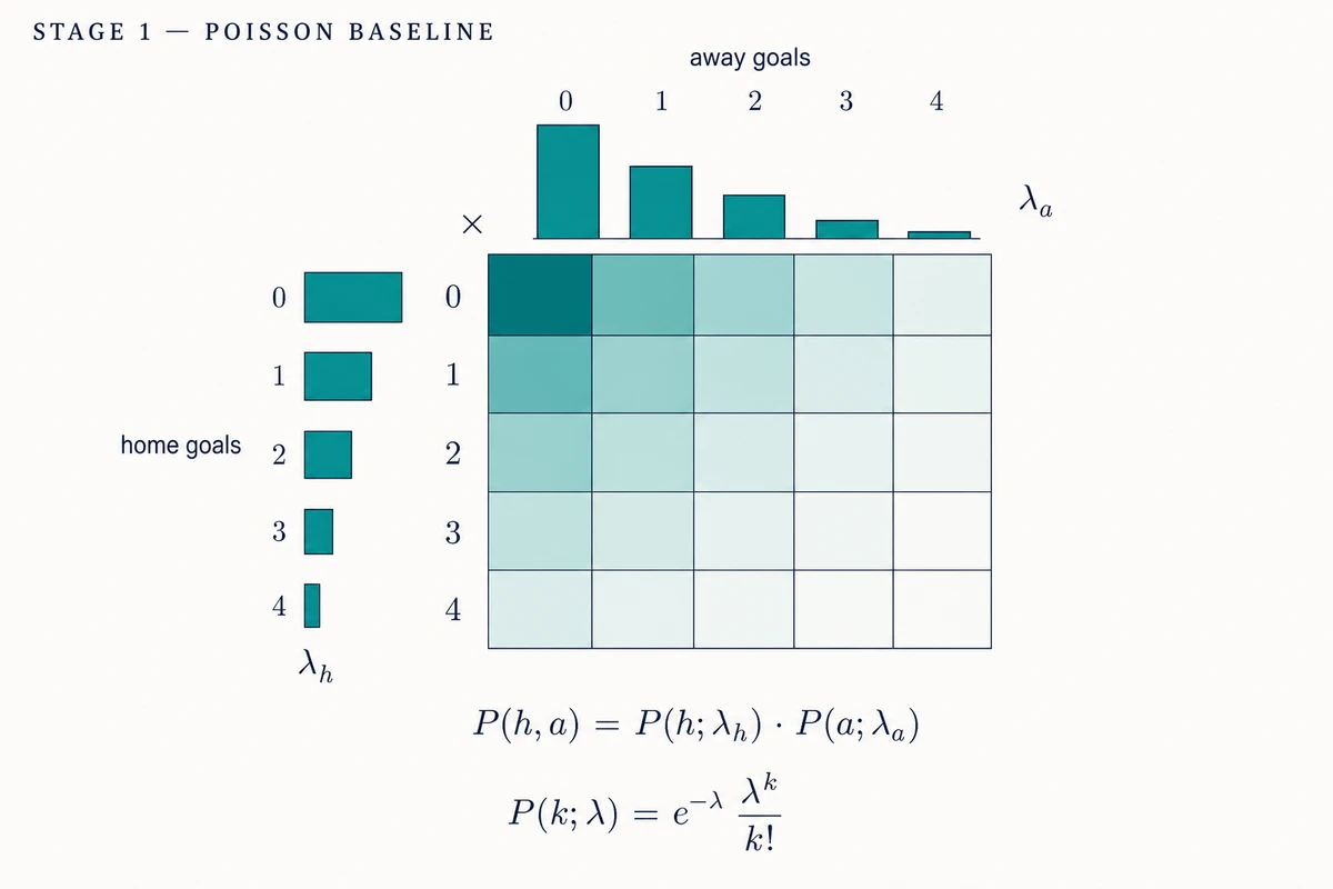
Each stage re-solves (λₕ, λₐ) against the same fair targets, so the score grid's stage switcher is a true before/after — flip Poisson / Dixon-Coles / 1X2 φ to see exactly what ρ and φ move.

Each period — full match, 1st half, 2nd half — is its own inversion from its own quotes. Markets that need goal timing, scoring method, in-match trajectory, or both halves at once (Half Time/Full Time, Highest Scoring Half, First/Next Goal, …) are out of scope here; see the Markets reference for the full catalog.

Primary Quotes

Handicap (Malay)

LineHomeAway

Total (Malay)

LineOverUnder

Dixon-Coles

ρ

1X2 quote (Decimal) optional · φ draw fit

Home1DrawXAway2

↑/↓ steps a field, Shift steps bigger; on a Malay pair the partner moves the opposite way. Handicap/Total ladders use your line ±0.25; team-total, 3-way and which-team lines are illustrative — probabilities are exact given λ.

Valid inputs: Malay in [−1, +1] and never 0, 1X2 decimals above 1, and each book must carry margin (implied probabilities summing over 1).

λₕ 1.7191λₐ 1.0155λ_total 2.7346φ 0.2098round-trip Δp 7.1e-8 / 3.1e-8 / 1.2e-10draw 0.2700 → 0.2995grid N=8 · Poisson → Dixon-Coles → 1X2 φ

Score grid — P(home = h, away = a) ×100

λₕ 1.7191λₐ 1.0155φ 0.2098draw 0.2995

	A=0	A=1	A=2	A=3	A=4	A=5	A=6	A=7	A=8
H=0	8.75	5.18	3.17	1.07	0.27	0.06	0.01	0.00	0.00
H=1	9.51	14.30	5.46	1.85	0.47	0.10	0.02	0.00	0.00
H=2	9.10	9.24	5.67	1.59	0.40	0.08	0.01	0.00	0.00
H=3	5.21	5.29	2.69	1.10	0.23	0.05	0.01	0.00	0.00
H=4	2.24	2.27	1.15	0.39	0.12	0.02	0.00	0.00	0.00
H=5	0.77	0.78	0.40	0.13	0.03	0.01	0.00	0.00	0.00
H=6	0.22	0.22	0.11	0.04	0.01	0.00	0.00	0.00	0.00
H=7	0.05	0.06	0.03	0.01	0.00	0.00	0.00	0.00	0.00
H=8	0.01	0.01	0.01	0.00	0.00	0.00	0.00	0.00	0.00

home win draw away winshade ∝ probability

MarketHandicapOver/UnderHome Over/UnderAway Over/Under1X2Correct ScoreDraw No BetOdd/EvenHome Odd/EvenAway Odd/EvenMyanmar HandicapMyanmar Over/UnderDouble ChanceClean SheetTo Win to NilBoth/One/Neither Teams to ScoreWinning Margin3-Way HandicapExact TotalRange TotalWhich Team Will Win By X+21 in scope

Multi-way (Shin)

Outcome	Odds
Home	1.928
Draw	3.167
Away	4.641

How these numbers are computed

1 · Strip the bookmaker margins — Power (two-way) · Shin (three-way)

A two-way Malay price converts to decimal ($d = 1 + m$ if $m > 0$, else $d = 1 - 1/m$), which implies a probability $q = 1/d$; the two sides sum to an overround $Q > 1$. The Power method finds the exponent $x$ that deflates them to a fair pair $p_i = q_i^{1/x}$, and the stripped (margin-free) decimal odds are the reciprocals $1/p_i$. The three-way 1X2 needs a different deflation — Shin (the formula is in step 5) — but lands in the same table shape. The fair numbers are the constraints the solver must reproduce.

Handicap -0.50 → P(home covers -0.50)

	Home	Away
Malay quote	+0.96	+0.96
Decimal $d$	1.9600	1.9600
Implied $q = 1/d$	0.5102	0.5102
Fair $p = q^{1/x}$	0.5000	0.5000
Fair decimal $1/p$	2.0000	2.0000

overround Q = 1.0204 → solve $q_1^{1/x} + q_2^{1/x} = 1$ → x = 0.9709 → fair P(home covers) = 0.5000

Total 2.50 → P(over 2.50)

	Over	Under
Malay quote	+0.95	+0.95
Decimal $d$	1.9500	1.9500
Implied $q = 1/d$	0.5128	0.5128
Fair $p = q^{1/x}$	0.5000	0.5000
Fair decimal $1/p$	2.0000	2.0000

overround Q = 1.0256 → solve $q_1^{1/x} + q_2^{1/x} = 1$ → x = 0.9635 → fair P(over) = 0.5000

1X2 (Decimal) → P(home win), P(draw), P(away win) — Shin

	Home	Draw	Away
Decimal quote $d$	1.8900	3.1300	4.7000
Implied $q = 1/d$	0.5291	0.3195	0.2128
Fair $p$ (Shin)	0.5060	0.2995	0.1945
Fair decimal $1/p$	1.9762	3.3389	5.1420

overround Q = 1.0614 → bisect Shin’s insider fraction z until $\textstyle\sum p_i = 1$ (step 5) → z = 0.0308 → fair draw = 0.2995, the φ target

Try the strips standalone — Margin — two-way (Power) · Margin — multi-way (Shin): the same math on any quotes, with the bisection narrated.

2 · Size — recover λ_total from the Total

Step 1 left three fair targets, and the model has matching knobs — the scoring rates $\lambda_h, \lambda_a$ plus the diagonal lift φ (step 5). Model each side’s goals as Poisson — $P(k;\lambda) = e^{-\lambda}\lambda^{k}/k!$ — and independent. Independent Poissons add — $X + Y \sim \mathrm{Poisson}(\lambda_h + \lambda_a)$ — so the match total depends only on $\lambda_{\text{total}} = \lambda_h + \lambda_a$: the Total quote pins the match size on its own, before caring who scores (step 3’s job). Every line class settles by the same rule (the line rules below): take the win mass $W$ and push mass $R$ of that one total — point masses $P(\text{total} = t) = e^{-\lambda}\lambda^{t}/t!$ — and the fair over-probability is $W/(1-R)$. That makes size a one-dimensional root-find, laid out below in the order a solver runs it — target, search, then the evaluation every iteration repeats:

target (step 1): $$p^{\ast}_{\text{over}} \;=\; \text{fair } P(\text{over } 2.50) \;=\; 0.5000$$

search: $$\text{bisect } \lambda_{\text{total}} \in [0.02,\, 8] \;\text{ until }\; W/(1-R) = p^{\ast}_{\text{over}} \;\Rightarrow\; \lambda_{\text{total}} = 2.6743$$

Each trial λ is scored the same way — the settlement rule evaluated under Poisson(λ). These are the figures a re-implementation should reproduce at the converged $\lambda = \lambda_{\text{total}} = 2.6743$: first each component line’s Poisson masses, then the weighted $W$ and $R$, then the fair check against the target:

$$P(\text{total} > 2.50) \;=\; 1 - \textstyle\sum_{t=0}^{2} \tfrac{e^{-\lambda}\lambda^{t}}{t!} \;=\; 0.5000 \qquad P(\text{total} = 2.50) \;=\; 0 \;\; \text{(totals are integers)}$$

$$W = P(\text{total} > 2.50) = 0.5000$$

$$R = P(\text{total} = 2.50) = 0.0000$$

$$\text{fair } P(\text{over } 2.50) \;=\; \frac{W}{1-R} \;=\; \frac{0.5000}{1 - 0.0000} \;=\; 0.5000 \;=\; p^{\ast}_{\text{over}} \;\; \checkmark$$

$$\Longrightarrow\;\; \lambda_{\text{total}} = 2.6743$$

(Additivity is exact only for the plain independent-Poisson grid, so this λ is the Poisson stage’s; the τ and φ adjustments of the later stages perturb it, so each re-solves size and split jointly against the same targets — all the recovered λ’s land in the per-stage tables (steps 4–5).)

Line rules — over wins ⟺ $h + a > T$; an exact hit ($h + a = T$) is a push: the stake refunds, so a two-way fair probability renormalizes it away, $\text{fair} = W/(1-R)$ (win mass over non-push mass). A .5 line cannot push, so $R = 0$ and the formula degenerates to $\text{fair} = W$ — same rule, not a shortcut method; a quarter line (±0.25, ±0.75, …) puts half the stake on each neighbouring line, so $W$ and $R$ are the ½-weighted sums over the two components. The same settlement applies to the Handicap (step 3) and the priced ladders (step 6).

3 · Split — recover λₕ and λₐ from the Handicap

The Handicap decides who scores them — and settling it needs the full scoreline distribution, the score grid: independence makes each cell $(h, a)$ a plain product of the two Poisson masses,

$$J[h][a] \;=\; P(\text{home} = h;\, \lambda_h) \cdot P(\text{away} = a;\, \lambda_a) \qquad h, a = 0 \ldots 8$$

— exactly the grid the score-grid panel’s Poisson stage displays. Hold $\lambda_{\text{total}}$ fixed and slide the home share $\lambda_h$ (with $\lambda_a = \lambda_{\text{total}} - \lambda_h$). Home covers ⟺ $h + L > a$, an exact $h + L = a$ is a push — step 2’s one rule again, with the masses now read off the grid: $W = \textstyle\sum_{h + L > a} J[h][a]$ and $R = \textstyle\sum_{h + L = a} J[h][a]$ (½-weighted across a quarter line’s two components), fair cover probability $W/(1-R)$ — which rises with $\lambda_h$, so the same solver shape applies:

target (step 1): $$p^{\ast}_{\text{cover}} \;=\; \text{fair } P(\text{home covers } -0.50) \;=\; 0.5000$$

search: $$\text{bisect } \lambda_h \in (0,\, \lambda_{\text{total}}) \;\text{ until }\; W/(1-R) = p^{\ast}_{\text{cover}} \;\Rightarrow\; \lambda_h = 1.6091,\;\; \lambda_a = \lambda_{\text{total}} - \lambda_h = 1.0652$$

At the converged split the grid masses and the fair check are:

$$W = P(h - 0.50 > a) = 0.5000$$

$$R = P(h - 0.50 = a) = 0.0000$$

$$\text{fair } P(\text{home covers } -0.50) \;=\; \frac{W}{1-R} \;=\; \frac{0.5000}{1 - 0.0000} \;=\; 0.5000 \;=\; p^{\ast}_{\text{cover}} \;\; \checkmark$$

$$\Longrightarrow\;\; \lambda_h = 1.6091 \qquad \lambda_a = 1.0652$$

The recovered pair $(\lambda_h,\, \lambda_a)$ is the Poisson stage’s chips in the grid panel — and with it both quotes are reproduced exactly. That closes the fit, but not the model: the two quotes pinned just two numbers, size and split, while step 6 prices whole ladders off the grid’s shape — and that shape so far rests entirely on the independence assumption. The next steps correct the shape where independence is known to fail, then re-solve so the quotes still hold: Dixon-Coles’ low-score τ (step 4), then the 1X2 draw lift φ (step 5).

4 · Dixon-Coles — re-solve with the low-score tilt τ

Steps 2–3 hit both targets exactly — so what is left? Infinitely many grids satisfy those same two constraints; the independent product is merely the simplest of them, and it is empirically wrong in one known corner: real matches produce slightly more 0-0 and 1-1, and fewer 1-0/0-1, than independence predicts (the Dixon-Coles finding). The fix multiplies exactly those four cells by a tilt τ driven by a correlation knob ρ. Note ρ is not recovered from your quotes — steps 2–3 already spent both of them — it is a modelling input, the ρ field in the Dixon-Coles section above (league-calibrated in practice). Negative ρ lifts 0-0/1-1 and trims 1-0/0-1; positive ρ the reverse; τ = 1 leaves everything else alone:

$$J[h][a] \;\mapsto\; J[h][a] \cdot \tau(h,a) \qquad \tau = 1 \;\text{everywhere except the four low-score cells}$$

with ρ = -0.10 at the re-solved pair (λₕ, λₐ) = (1.6331, 1.0411) from below:

$$\tau(0,0) \;=\; 1 - \lambda_h \cdot \lambda_a \cdot \rho \;=\; 1 - 1.6331 \times 1.0411 \times (-0.10) \;=\; 1.1700$$

$$\tau(0,1) \;=\; 1 + \lambda_h \cdot \rho \;=\; 1 + 1.6331 \times (-0.10) \;=\; 0.8367$$

$$\tau(1,0) \;=\; 1 + \lambda_a \cdot \rho \;=\; 1 + 1.0411 \times (-0.10) \;=\; 0.8959$$

$$\tau(1,1) \;=\; 1 - \rho \;=\; 1 - (-0.10) \;=\; 1.1000$$

The tilted grid is renormalized to $\textstyle\sum J = 1$ (ρ is valid only while every τ stays positive). That reshaping breaks the step 2–3 fit — the same λ pair now prices differently, because $W$ and $R$ are sums over a grid whose mass just moved. Nothing else changes: the targets stay step 1’s, the settlement rule stays $W/(1-R)$, and the same two nested bisections simply run again with the τ-tilted grid underneath. In the same solver order as steps 2–3:

targets (step 1, unchanged): $$p^{\ast}_{\text{over}} = 0.5000 \qquad p^{\ast}_{\text{cover}} = 0.5000$$

old pair on the τ-grid: $$(\lambda_h,\, \lambda_a) = (1.6091,\, 1.0652): \quad \text{fair } P(\text{over}) = 0.5000 \qquad \text{fair } P(\text{cover}) = 0.4882 \qquad \text{cover off target}$$

search: $$\text{bisect } \lambda_{\text{total}} \in [0.02,\, 8] \text{ and } \lambda_h \in (0,\, \lambda_{\text{total}}) \text{ exactly as in steps 2–3, } W \text{ and } R \text{ now summed off the } \tau\text{-grid}$$

check (new pair, τ-grid): $$\text{at } (\lambda_h,\, \lambda_a) = (1.6331,\, 1.0411)\!: \quad \text{fair } P(\text{over } 2.50) \;=\; \frac{W_{\tau}}{1-R_{\tau}} \;=\; \frac{0.5000}{1 - 0.0000} \;=\; 0.5000 \;=\; p^{\ast}_{\text{over}} \;\; \checkmark$$

$$\text{fair } P(\text{home covers } -0.50) \;=\; \frac{W_{\tau}}{1-R_{\tau}} \;=\; \frac{0.5000}{1 - 0.0000} \;=\; 0.5000 \;=\; p^{\ast}_{\text{cover}} \;\; \checkmark$$

$$\Longrightarrow\;\; (\lambda_h,\, \lambda_a): \; (1.6091,\, 1.0652) \;\xrightarrow{\;\tau,\;\rho \,=\, -0.10\;}\; (1.6331,\, 1.0411) \qquad \lambda_{\text{total}}: \; 2.6743 \to 2.6742$$

Step 3 ended on $\text{fair } P(\text{home covers } -0.50) = 0.5000$ with $\lambda_h = 1.6091$; step 4 ends on the same 0.5000 with $\lambda_h = 1.6331$. That is by construction, not coincidence: 0.5000 is the target — step 1’s $p^{\ast}_{\text{cover}}$ — and a bisection only stops when it lands there, so every ✓ line prints the same number no matter which grid sits underneath. The fair value is a function of two inputs, the grid and the λ pair; the λ’s differ precisely because the grid differs. Evaluate both pairs on both grids and the compensation becomes visible:

fair P(home covers -0.50)	product grid (step 3)	τ-grid, ρ = -0.10 (step 4)
step-3 pair (1.6091, 1.0652)	0.5000 ✓	0.4882 ✗
step-4 pair (1.6331, 1.0411)	0.5117 ✗	0.5000 ✓

Read it by row — same pair, swap the grid — and the tilt shows: at the step-3 pair, τ alone drags the cover value 0.5000 → 0.4882. Read it by column — same grid, swap the pair — and the repair shows: on the τ-grid, moving to the step-4 pair brings it back to 0.5000. Each grid has exactly one ✓ cell; tilting the grid moved the solution point, and finding its new location is all the step-4 bisection does. ρ itself never enters the settlement rule — it acts one layer down, inside the cells that $W$ and $R$ sum over: step 3’s $W$ is summed off the product grid, step 4’s $W_{\tau}$ off the τ-tilted grid (the subscript names the grid the sum runs over — it is not a power). For example the 1-0 cell (a τ cell) goes $J[1][0]: 0.1110 \to 0.1009 \quad (\tau(1,0) = 1 + \lambda_a \rho = 0.8959)$ while the re-split of λₕ vs λₐ moves the untouched cells by exactly enough that the aggregate lands back on the targets. The side-by-side grids at the end of this step show that recomposition cell by cell.

(The table tracks the cover value because at a total line of 2.50 all four τ cells sit on the under side, so the tilt’s net mass shift nearly cancels and fair $P(\text{over})$ barely moves — off target only past 4 dp. The visible repair is almost entirely on the cover side.)

Unroll the search — every bisection iteration

Outer loop — size. Each row takes the bracket midpoint as a trial $\lambda_{\text{total}}$, runs the full inner bisection (second table) to find the λₕ that restores the cover target on that trial’s τ-grid, then compares the resulting fair $P(\text{over})$ with $p^{\ast}_{\text{over}} = 0.5000$ to decide which half of the bracket survives:

k	lo	hi	trial λ_total	inner λₕ	fair P(over)	move
1	0.020000	8.000000	4.010000	2.286293	0.76319375	↓
2	0.020000	4.010000	2.015000	1.312023	0.32737692	↑
3	2.015000	4.010000	3.012500	1.798293	0.57955654	↓
4	2.015000	3.012500	2.513750	1.554844	0.45968894	↑
5	2.513750	3.012500	2.763125	1.676530	0.52167833	↓
6	2.513750	2.763125	2.638437	1.615675	0.49115104	↑
7	2.638437	2.763125	2.700781	1.646100	0.50653826	↓
8	2.638437	2.700781	2.669609	1.630887	0.49887476	↑
9	2.669609	2.700781	2.685195	1.638493	0.50271414	↓
10	2.669609	2.685195	2.677402	1.634690	0.50079635	↓
11	2.669609	2.677402	2.673506	1.632788	0.49983603	↑
12	2.673506	2.677402	2.675454	1.633739	0.50031630	↓
13	2.673506	2.675454	2.674480	1.633264	0.50007619	↓
14	2.673506	2.674480	2.673993	1.633026	0.49995612	↑
15	2.673993	2.674480	2.674236	1.633145	0.50001616	↓
16	2.673993	2.674236	2.674115	1.633085	0.49998614	↑
17	2.674115	2.674236	2.674176	1.633115	0.50000115	↓
18	2.674115	2.674176	2.674145	1.633100	0.49999364	↑
19	2.674145	2.674176	2.674160	1.633108	0.49999740	↑
20	2.674160	2.674176	2.674168	1.633111	0.49999927	↑
21	2.674168	2.674176	2.674172	1.633113	0.50000021	↓
22	2.674168	2.674172	2.674170	1.633112	0.49999974	↑
23	2.674170	2.674172	2.674171	1.633113	0.49999998	✓

Inner loop — split. At the converged $\lambda_{\text{total}} = 2.674171$, each row prices the τ-grid at $(\lambda_h,\; \lambda_{\text{total}} - \lambda_h)$ and checks fair $P(\text{cover})$ against $p^{\ast}_{\text{cover}} = 0.5000$:

j	lo	hi	trial λₕ	fair P(cover)	move
1	0.010000	2.664171	1.337085	0.35785478	↑
2	1.337085	2.664171	2.000628	0.67699314	↓
3	1.337085	2.000628	1.668857	0.51752852	↓
4	1.337085	1.668857	1.502971	0.43653752	↑
5	1.502971	1.668857	1.585914	0.47689072	↑
6	1.585914	1.668857	1.627385	0.49719266	↑
7	1.627385	1.668857	1.648121	0.50735869	↓
8	1.627385	1.648121	1.637753	0.50227491	↓
9	1.627385	1.637753	1.632569	0.49973356	↑
10	1.632569	1.637753	1.635161	0.50100418	↓
11	1.632569	1.635161	1.633865	0.50036886	↓
12	1.632569	1.633865	1.633217	0.50005120	↓
13	1.632569	1.633217	1.632893	0.49989238	↑
14	1.632893	1.633217	1.633055	0.49997179	↑
15	1.633055	1.633217	1.633136	0.50001150	↓
16	1.633055	1.633136	1.633096	0.49999164	↑
17	1.633096	1.633136	1.633116	0.50000157	↓
18	1.633096	1.633116	1.633106	0.49999661	↑
19	1.633106	1.633116	1.633111	0.49999909	↑
20	1.633111	1.633116	1.633113	0.50000033	↓
21	1.633111	1.633113	1.633112	0.49999971	↑
22	1.633112	1.633113	1.633113	0.50000002	✓

move: ↑ = fair below target → keep the upper half (lo = mid) · ↓ = above → keep the lower half (hi = mid) · ✓ = |fair − target| < 1e-7 (the dc-stage tolerance; 60-iteration cap). The two final rows land on (1.6331, 1.0411) — step 4’s pair in the ⟹ line above. Every earlier outer row ran this same inner loop against its own trial λ_total; the inner table shown is the one belonging to the winning size.

Reading the repair: each miss has its own knob — a Total miss moves the size (step 2’s bisection on λ_total), a Handicap miss moves the split (step 3’s on λₕ). Here the tilt knocked the cover target off harder (by 0.0118, vs 0.0000 for the over) — ρ < 0 parks its extra mass on the draw cells 0-0/1-1, and on a home -0.50 line a draw is a lost cover — so the correction lands mainly in the split: λₕ +0.0240, λₐ −0.0241, λ_total −0.0001.

Both stages so far are the same nested solve (steps 2–3), each run on its own grid:

Stage	λₕ	λₐ	λₕ+λₐ	Δ cover	Δ over
Poisson	1.6091	1.0652	2.6743	8.4e-9	1.6e-10
Dixon-Coles	1.6331	1.0411	2.6742	1.9e-8	2.4e-8

These rows are the score-grid panel’s λ chips; the Δ’s are each stage’s achieved |model − target| residuals — the convergence check. One optional constraint remains before the markets price — step 5.

Side by side, the tilt becomes visible — the low-score corner of both grids, every cell shaded by how Dixon-Coles moved it (green = up, red = down; hover a cell for the exact before → after, and click any Dixon-Coles cell for its full derivation from the Poisson pieces):

Poisson (λₕ 1.6091 · λₐ 1.0652)

	A=0	A=1	A=2	A=3	A=4	A=5
H=0	0.0690	0.0735	0.0391	0.0139	0.0037	0.0008
H=1	0.1110	0.1182	0.0629	0.0223	0.0060	0.0013
H=2	0.0893	0.0951	0.0506	0.0180	0.0048	0.0010
H=3	0.0479	0.0510	0.0272	0.0096	0.0026	0.0005
H=4	0.0193	0.0205	0.0109	0.0039	0.0010	0.0002
H=5	0.0062	0.0066	0.0035	0.0012	0.0003	0.0001

Dixon-Coles, re-solved (λₕ 1.6331 · λₐ 1.0411)

	A=0	A=1	A=2	A=3	A=4	A=5
H=0	0.0807	0.0601	0.0374	0.0130	0.0034	0.0007
H=1	0.1009	0.1290	0.0610	0.0212	0.0055	0.0011
H=2	0.0920	0.0957	0.0498	0.0173	0.0045	0.0009
H=3	0.0501	0.0521	0.0271	0.0094	0.0025	0.0005
H=4	0.0204	0.0213	0.0111	0.0038	0.0010	0.0002
H=5	0.0067	0.0070	0.0036	0.0013	0.0003	0.0001

mass up vs Poisson mass down the four τ cellsshade ∝ √|Δ| · both grids share the same shading · shown 0–5, higher cells barely move

5 · Lift the diagonal to the 1X2 draw (φ · Method A) — optional

The 1X2 is a three-way book, so Shin stripped it in step 1: with implied $q_i = 1/d_i$ and overround $Q = \textstyle\sum q_i$, Shin’s insider fraction $z$ deflates each side to

$$p_i(z) \;=\; \frac{\sqrt{z^{2} + 4(1-z)\,q_i^{2}/Q\,} - z}{2(1-z)} \qquad \text{bisect } z \in [0,1) \text{ until } \textstyle\sum p_i = 1 \;\Rightarrow\; z = 0.0308$$

giving fair $P(\text{home})\, 0.5060$, $\text{draw}\, 0.2995$, $P(\text{away})\, 0.1945$. The handicap already fixes the win sides; the draw — the grid’s diagonal $\textstyle\sum_k J[k][k]$ — is the new constraint. Multiplying every equal-score cell by $(1 + \varphi)$, renormalizing the grid to $\textstyle\sum J = 1$, and re-solving $(\lambda_h, \lambda_a)$ so the Handicap and Total still hold, a third bisection lands φ on the draw (Method A: one flat factor across the whole diagonal, i.e. per-cell weights $w_k = 1$). The “two-input draw” below is the φ = 0 grid’s diagonal mass — the Dixon-Coles stage’s draw chip in the score-grid panel:

$$\underbrace{0.2700}_{\text{two-input draw}} \;\xrightarrow{\;\varphi \,=\, 0.2098\;}\; \underbrace{0.2995}_{\text{1X2 draw target}} \qquad \Delta = 1.2 \times 10^{-10}$$

Unroll the φ search — every bisection iteration

Third loop — the draw. Each row lifts every equal-score cell by $(1 + \varphi)$ at its trial φ, renormalizes, re-solves $(\lambda_h,\, \lambda_a)$ against the Handicap and Total targets — the entire two-level bisection unrolled in step 4, now on the lifted grid — and reads the solved grid’s diagonal $\textstyle\sum_k J[k][k]$ against the draw target $0.2995$. Bracket: the two-input draw 0.2700 < target → inflate it: φ ∈ [0.0000, 1.0000]:

i	lo	hi	trial φ	λₕ	λₐ	draw	move
1	0.000000	1.000000	0.50000000	1.829378	0.979786	0.332246282	↓
2	0.000000	0.500000	0.25000000	1.734935	1.010530	0.304544039	↓
3	0.000000	0.250000	0.12500000	1.685002	1.025884	0.288248091	↑
4	0.125000	0.250000	0.18750000	1.710206	1.018220	0.296623306	↑
5	0.187500	0.250000	0.21875000	1.722629	1.014378	0.300638584	↓
6	0.187500	0.218750	0.20312500	1.716432	1.016300	0.298644906	↑
7	0.203125	0.218750	0.21093750	1.719534	1.015339	0.299645194	↓
8	0.203125	0.210938	0.20703125	1.717984	1.015820	0.299145939	↑
9	0.207031	0.210938	0.20898438	1.718760	1.015579	0.299395765	↑
10	0.208984	0.210938	0.20996094	1.719147	1.015459	0.299520543	↓
11	0.208984	0.209961	0.20947266	1.718953	1.015519	0.299458184	↑
12	0.209473	0.209961	0.20971680	1.719050	1.015489	0.299489334	↑
13	0.209717	0.209961	0.20983887	1.719099	1.015474	0.299504958	↓
14	0.209717	0.209839	0.20977783	1.719074	1.015482	0.299497180	↑
15	0.209778	0.209839	0.20980835	1.719087	1.015478	0.299501031	↑
16	0.209808	0.209839	0.20982361	1.719092	1.015476	0.299503028	↑
17	0.209824	0.209839	0.20983124	1.719096	1.015475	0.299503960	↓
18	0.209824	0.209831	0.20982742	1.719094	1.015475	0.299503475	↑
19	0.209827	0.209831	0.20982933	1.719095	1.015475	0.299503734	↓
20	0.209827	0.209829	0.20982838	1.719094	1.015476	0.299503607	↑
21	0.209828	0.209829	0.20982885	1.719095	1.015475	0.299503651	↓
22	0.209828	0.209829	0.20982862	1.719095	1.015475	0.299503610	↑
23	0.209829	0.209829	0.20982873	1.719095	1.015475	0.299503631	✓

move: ↑ = draw below target → keep the upper half (lo = mid) · ↓ = above → keep the lower half (hi = mid) · ✓ = |draw − target| < 1e-9 (48-iteration cap). The ✓ row is the stage’s result: φ = 0.2098 with the re-solved pair (1.7191, 1.0155) — the 1X2 φ chips in the grid panel and the last row of the table below. Every row re-ran the whole step-4 nest at its own trial φ.

The φ stage re-runs the same nested solve with this third constraint attached, completing step 4’s per-stage table:

Stage	λₕ	λₐ	λₕ+λₐ	φ	Δ cover	Δ over	Δ draw
Poisson	1.6091	1.0652	2.6743	—	8.4e-9	1.6e-10	—
Dixon-Coles	1.6331	1.0411	2.6742	—	1.9e-8	2.4e-8	—
1X2 φ	1.7191	1.0155	2.7346	0.2098	7.1e-8	3.1e-8	1.2e-10

Every market below prices off the last row’s grid; Δ draw is the φ bisection’s achieved residual.

Consistency — the Handicap owns the tilt, so the 1X2 win legs are a cross-check, not a constraint: model P(home win) 0.5000 vs 1X2 0.5060, P(away win) 0.2005 vs 0.1945. A large gap means the three quotes disagree (different books or times). One draw number fixes the diagonal’s level only — the 2-2/3-3/4-4 shape rides on the flat wₖ; pin it with correct-score quotes. Flat wₖ also lifts only even totals (every k-k totals 2k), so the fit nudges Odd/Even and Exact-Total toward even — Method A is not draw-isolated. ρ and φ both lift 0-0/1-1, so φ absorbs part of ρ — the two are not independently interpretable; flip the Dixon-Coles and 1X2 φ stages in the grid panel to see φ’s residual move.

6 · Read “1X2” off the score grid

With λₕ, λₐ and φ fixed, the last stage’s grid $J[h][a]$ (step 5) is fully determined — the score-grid panel above — and every market probability is just a sum of its matching cells. Home sums every grid cell with home > away, Draw the diagonal, Away the cells with home < away.

Outcome	Σ from grid	Fair	Priced dec
Home	0.5000	0.5000	1.928
Draw	0.2995	0.2995	3.167
Away	0.2005	0.2005	4.641

Raw masses are normalized to Σ = 1, then inflated by Shin to overround 1 + 0.05 — the insider model run forward: $q_i = S \cdot t_i$ with $t_i = \sqrt{p_i((1-z)p_i + z)}$ and $S = \textstyle\sum t_i$, bisecting $z$ until $\textstyle\sum q_i = 1.05$ (this run: $z = 0.0251$).

7 · Implementation notes — nesting, brackets, normalization

targets   tH = powerStrip(HCP pair)      # fair P(home covers L)         — step 1
          tT = powerStrip(Total pair)    # fair P(over T)                — step 1
          tD = shinStrip(1X2).draw       # fair P(draw); Method A only   — step 5

bisect φ ∈ (−1, ∞)                       # outermost; skip (φ = 0) with no 1X2
  bisect λ_total ∈ [0.02, 8]             # size — step 2
    bisect λₕ ∈ (0, λ_total)             # split — step 3; λₐ = λ_total − λₕ
      J = Poisson(λₕ, λₐ) on 0…N         # ×τ + renorm (DC — step 4); φ stage: diag ×(1+φ) + renorm
    until fairHcp(J, L) = tH             # line rules — step 2
  until fairTot(J, T) = tT
until Σₖ J[k][k] = tD

The grid panel’s stages run this same nest with the adjustments off/on — Poisson: neither, Dixon-Coles: τ only, 1X2 φ: both. Every residual is monotone in its knob — cover rises with λₕ, over with λ_total, draw with φ — so plain bisection converges: 48–60 iterations per loop at tolerances 1e-9…1e-7 (the round-trip Δp above is this run’s achieved error). The φ bracket doubles upward from [0, 1], or flips to (−1, 0] when the two-input draw already exceeds the 1X2 target. The grid truncates at N = 8: the plain Poisson grid is not renormalized, the τ- and φ-adjusted grids are, and every market group renormalizes its outcome masses to Σ = 1 before its margin is applied — that absorbs the truncation loss. The executable reference for all of the above is docs/src/lib/odds/core.ts + markets.ts, held to the original simulator by the golden-master test in docs/src/lib/odds/__tests__/.